Does Harris corner detector finds corners? (Intuitive explanation to Harris corner detector)

I want to take a short break of the series on pentomino recognition from scanned paper. This week I would like to explain Harris corner detector.  Most of the explanations that I found on the web and in books tend to focus on the spatial difference between templates, the derivation of Taylor polynomial and explanation about covariance matrix. While this explanation is technically correct, in my opinion, it is hardly intuitive. Moreover, it does not show an important step of the algorithm, which can be used for more specific objects detection. I got this intuition after seeing this video.

But before that, test yourself. Given the following image, what places do you think that Harris corner detector will find? Try to do this without actually running the detector on the image.

After reading the rest of this post, you will be able to answer this question quickly and with confidence. By the way, if you think that the answer is only the corners of the checkerboard, keep on reading; It might be a surprise for you, Harris will prefer many other points to these corners.

In order to understand the algorithm, please consider the following pseudo code:

1. For some point (x,y)
2. Take a small rectangular region of interest around the point.
3. Find edges, in x and y direction. This is done by doing convolution with the appropriate templates. This  yields two images, Ix and Iy.
4. Draw a scatter plot of Ix(x’,y’) and Iy(x’,y’), of all the points (x’,y’) in the region of interest.

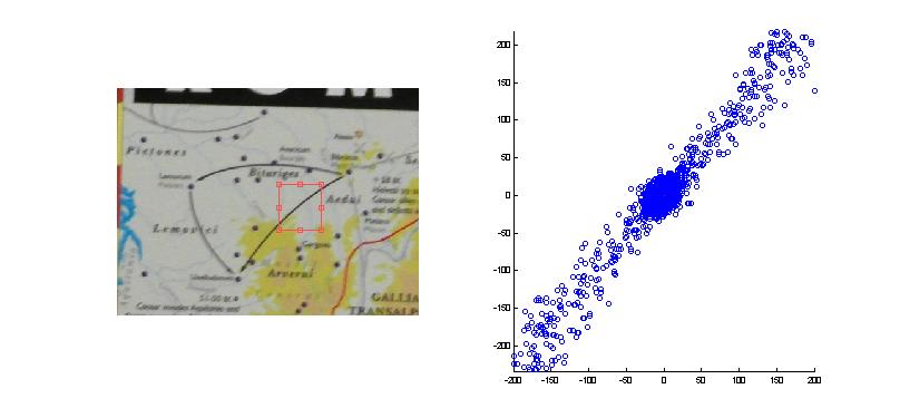
I wrote a small Matlab code that you can download, move the region of interest on the image (it is a draggable and moveable rectangle), and see what happens. The code responds quite quickly for a movement of a small region of interest. If you are intersted in the graphical aspect of how to re-draw scatter plot fastly, you can read this.

function HarrisExplanation
       % See explanation here : https://matlabcorner.wordpress.com/2012/11/17/does-harris-corner-detector-finds-corners-intuitive-explanation-to-harris-corner-detector/     
	im = imread('https://matlabcorner.wordpress.com/wp-content/uploads/2012/11/checkersandbooksmall.jpg');
	figure();
    a1 = subplot(1,2,1);
    a2 = subplot(1,2,2);
	xlim(a2,[-100 100]);
	ylim(a2,[-100 100]);

    imshow(im,'Parent',a1);
    initialPosition = [10 10 100 100];
    rectHandle = imrect(a1,initialPosition);

	scatterHandle = scatter([],[]);
	hold(a2,'on');
	v1 = plot(a2,0,0,'r');
	v2 = plot(a2,0,0,'r');

    rectHandle.addNewPositionCallback( @(pos)Callback(pos,scatterHandle,a2,v1,v2,im));
end

function Callback(position,scatterHandle,a2,v1,v2,im)
    x1 = position(1);
    y1 = position(2);
    x2 = position(1) + position(3);
    y2 = position(2) + position(4);

    thumbnail = double(im( round(y1:y2),round(x1:x2),2));
	dx = [-1 0 1;
		  -1 0 1;
		  -1 0 1];
	dy = dx';
	Ix = conv2(thumbnail,dx,'valid');
	Iy = conv2(thumbnail,dy,'valid');
	set(scatterHandle,'XData',Ix(:),'YData',Iy(:));
	A = [ sum(Ix(:).*Ix(:)) sum(Ix(:).*Iy(:)); sum(Ix(:).*Iy(:)) sum(Iy(:).*Iy(:)) ];
	[V,vals] = eig(A);

	lambda(1) = vals(1,1);
	lambda(2) = vals(2,2);
	
	lambda = lambda./max(lambda);

	set(v1,'XData',[0 V(1,1)*100*lambda(1)],'YData',[0 V(1,2)*100*lambda(1)]);
	set(v2,'XData',[0 V(2,1)*100*lambda(2)],'YData',[0 V(2,2)*100*lambda(2)]);

	xlim(a2,[-200 200]);
	ylim(a2,[-200 200]);
	axis(a2,'equal');
end

Here is an example of some regions of interest, and their scatter plots. The first image shows what happens in a region that is almost uniform. All of the points are concentrated in the middle of the plot.  When thinking about it in polar coordinates, all of the points have small magnitude.

The next image is an example of an area with all sort of edges. There are edges in all kind of direction, and with high magnitude.

If we take a look at a circle, we will see a similar behavior. On the circle arc, almost any angle exists, with high magnitude.

The image below has an edge in a specific direction. The scatter plot now shows an interesting behavior, it has points only with the angle of the edge, or the opposite angle. That is because there are white->black edges and black->white edges. All sorts of magnitudes exist, because the image has noise.

Taking a look at the checkerboard edge, we see only one specific direction. That is because the edges are all black->white.

At the corner of the checkerboard you will see a cross shape in the scatter plot.

Now how would you separate the regions of interest to the ones that either have no edges or edges in one direction? One possible way is to calculate the covariance matrix of the point and check that there are two high eigenvalues.The non-centered covariance matrix is defined as:

Where the <> brackets denote a sum over all possible values.

(Usually the covariance matrix is defined in terms of central moments, that is the data mean value is zero, however, here is not the case). If you don’t know what the covariance matrix is, just take a look at the following image:

The arrows direction are the eigenvectors of this matrix, and their length is the eigenvalues of the covariance matrix. Those of you who have heard about principal component analysis will have easy time understanding what is going on here. (More information about it is available here.)

At this point, Shi-Tomasi and Harris vary a little bit. Shi-Tomasi find the minimal eigenvalue and Harris uses some heuristic to save computation time. Also, in the actual algorithm, the matrix is weighted according to the distance of the point from the center of the region of interest.

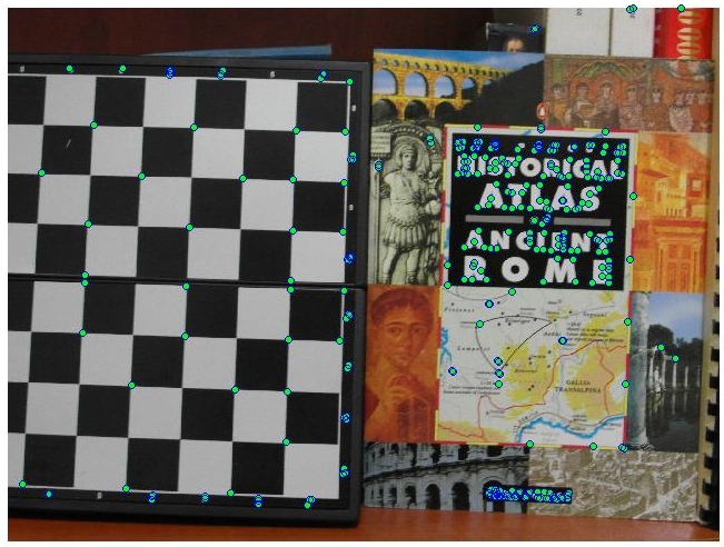
After saying all of this, let’s take a look at the Shi-Tomasi corner detector variation of the image above. We will plot only values with large enough response. I did some thresholding and I am plotting the centers of the blobs that are left after.

Here is the relevant Matlab code. Matlab uses by default 5×5 window for Harris, with Gaussian weights.

c = cornermetric(im(:,:,2),'MinimumEigenvalue');
figure;imagesc(c);
th = 0.3;
largeEnoughCorners = c > th * max(c(:));
centroids = regionprops(largeEnoughCorners,'Centroid');
centers = cat(1,centroids.Centroid);
figure;imshow(im);hold('on');scatter(centers(:,1),centers(:,2),'SizeData',60,'MarkerFaceColor','g');

Now, after understanding the intuition behind the algorithm, you should not be surprised when you see the center of the letter “O” found, even though it does not look like a corner. The letter “O” just has edges with high magnitude and at least two orthogonal directions.

In fact Harris does not find corners! Well, at least not in the everyday meaning of the word. It finds “feature points”, these are places that have low self similarity. That depends on the size of the window, but don’t expect to find only the corners of the checkerboard.

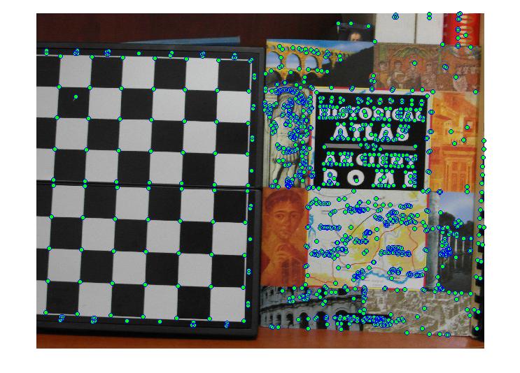
In order to get a better chance of detecting the corners of the checkerboard, we should increase Harris’s region of interest and decrease the threshold.

c = cornermetric(im(:,:,2),'MinimumEigenvalue','FilterCoefficients', fspecial('gaussian',[1 31],1.5));
figure;imagesc(c);
th = 0.1;
largeEnoughCorners = c > th * max(c(:));
centroids = regionprops(largeEnoughCorners,'Centroid');
centers = cat(1,centroids.Centroid);
figure;imshow(im);hold('on');scatter(centers(:,1),centers(:,2),'SizeData',60,'MarkerFaceColor','g');

Now the result is:

In the next post I will explain how to find only the corners of the checkerboard. You can use the “follow” button to subscribe by e-mail.